DPRODUCT Function in Excel: Explained
In the article, you will learn how to use the DPRODUCT function in Excel.
What is the DPRODUCT function in Excel?
The DPRODUCT function is a database function in Excel that returns the product of the values in a field (column) of records in a list or database that match the conditions you specify.
When is the DPRODUCT function in Excel beneficial?
The DPRODUCT function in Excel is beneficial when you need to multiply the values in a specific field or column of records in a database or a list that meets certain conditions. This can be really useful in specific contexts such as:
- Inventory management: You can use DPRODUCT to calculate the total value of specific types of items in your inventory. You can set criteria based on product type, product category, location, and other factors.
- Financial Analysis: In financial analysis, the DPRODUCT function can be used to calculate the product of values such as interest rates or growth rates for a specific set of time periods or conditions.
Understanding the syntax of the Excel DPRODUCT function
The syntax for the DPRODUCT function is the following:
Database: This required argument points to the cell range of the data, including the column labels.
Field: This required argument refers to the column that will have the product calculated. It can be the column name in quotes or a numerical reference to the column (where 1 represents the first column in the database, 2 represents the second, and so forth).
Criteria: This is a required argument that signifies the cell range containing the conditions that should be used for the product calculation. The cells in this range should feature column headers that match those in your database.
How to use the Excel DPRODUCT function
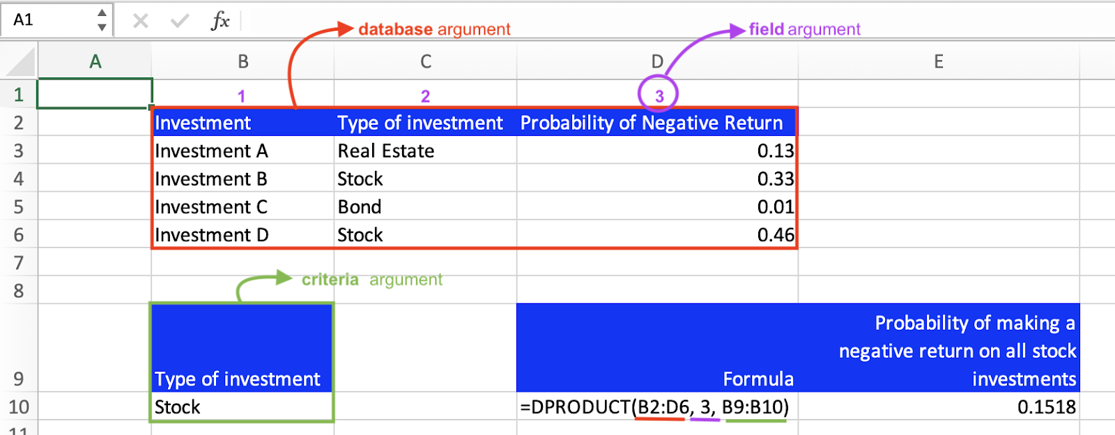
Suppose you had a database of investments that listed the type of investment and the probability of a negative return and you wanted to figure out the probability that all your stock investments would have negative returns. Below is an image showing this example.

Let's break down this example as seen throughout the annotations of the image. The database argument is the entire range of cells, including the column headers. The field argument in this case is “3”, so the product calculation takes place on the probability of a negative return column. As mentioned earlier, the field argument can be written as either the number column in the database or the column header, so in this example it could also have been plugged in as “Probability of Negative Return”. The criteria argument is a separate range of cells that specifies the conditions that should be applied to the product calculation. So in this formula we specify we only want the product of the stock investments.
Go to the page LiveFlow‘s How to Guides to find more information about Excel and Google Sheets formulas and tips that were not covered here.

