Dependent Drop-down List in Google Sheets: Explained
In this article, you will learn how to create a dependent drop-down menu in Google Sheets.
What is a dynamic drop-down menu in Google Sheets?
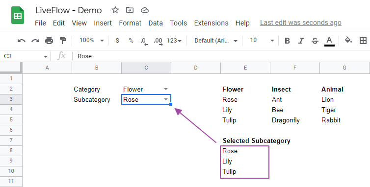
A dynamic drop-down list means its choices are determined by another drop-down list it refers to. For example, assume you have three categories, Flower, Insect, and Animal. Each category has three subcategories: Rose, Lily, and Tulip for Flower; Ant, Bee, and Dragonfly for Insect; and Lion, Tiger, and Rabbit for Animal. You have two drop-down lists, one for the category and the other for the subcategory. The values in the pull-down menu for the subcategory change depending on the choice in the drop-down menu when the second drop-down menu is called dependent or dynamic drop-down list.
How do I create a dependent list in Google Sheets?
- Prepare a list of choices for the drop-down menus.
- Create the first drop-down list.
- Generate Named Ranges for ranges containing values for the second pull-down menu. The ranges' names must be those of the values in the first pull-down list.
- Insert the INDIRECT formula referring to the first drop-down list, whose output the second pull-down list refers to.
- Create the second drop-down list.
Learn the steps above by looking at the specific example below. Assume we will create the dependent list described in the upper section. Category items will be in the first drop-down list, and subcategories will change depending on the first choice.
- Categories: Flower / Insect / Animal
- (When Flower is chosen) Subcategories 1: Rose, Lily, and Tulip
- (When Insect is selected) Subcategories 2: Ant, Bee, and Dragonfly
- (When Animal is picked up) Subcategories 3: Lion, Tiger, and Rabbit
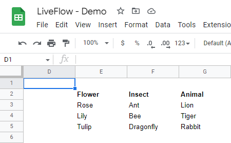
Step 1: You need to prepare a list of choices summarizing the information above (or you can type them directly in the “Data Validation” window).
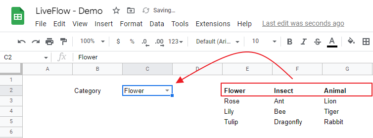
Step 2: Select E2:G2 as a range for the first drop-down menu. Check the first pull-down list is created correctly. (If you don’t know how to create a drop-down menu, check this article - (i) List from a range under the “How to do data validation in Google Sheets” section)
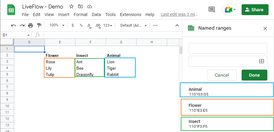
Step 3: Create Named Ranges by category, which is utilized in the next step. Select E3:E5, F3:F5, and G3:G5 for Flower subcategories, Insect ones, and Animal ones, respectively. Ensure you name the ranges after the categories (Flower, Insect, and Animal).
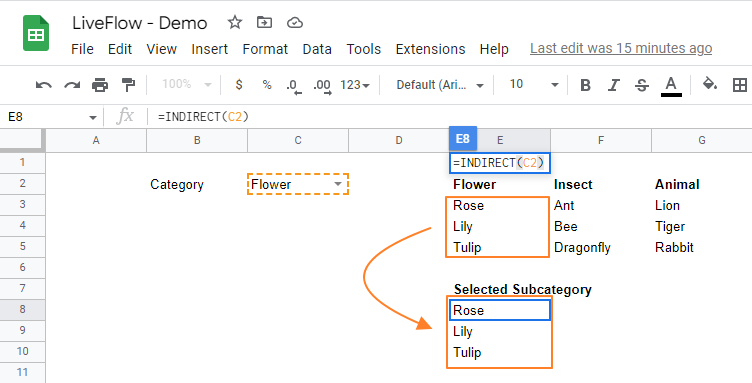
Step 4: Insert an INDIRECT function referring to the cell which contains the first drop-down list. If it works properly, combined with the named ranges, the INDIRECT formula should show one of the ranges containing subcategory names for the category selected in the first drop-down list. In this case, as “Flower” is chosen in the first pull-down menu, the INDIRECT presents its subcategory names.
Step 5: Create the second drop-down list by referring to the range the INDIRECT formula shows. Now you have the dependent pull-down menu. Ensure it works correctly by switching your choice in the first drop-down menu. If you change its choice, the content of the second pull-down list should change accordingly. (Note a value chosen from the previous first list in C3 remains unchanged when the first drop-down menu changes. You need to change the subcategory manually by choosing one item from the updated Subcategory list)
How do I link a drop-down list to another worksheet in Google Sheets?
- Copy the existing drop-down menu.
- Paste it into another worksheet in the same file.
- The same data validation rule is applied to the copied list.

