XLOOKUP Function in Excel: Explained
In this article, you will learn how to use the XLOOKUP formula in Excel.
What is the XLOOKUP formula in Excel?
The XLOOKUP function in Excel allows you to search for a value in a column / row and returns a corresponding value from the same position in another column / row. It is designed to be a more flexible and versatile replacement for the VLOOKUP and HLOOKUP functions.
XLOOKUP function was introduced in Excel 365.
Uses of XLOOKUP formula in Excel
The XLOOKUP function in Excel has several practical uses and can be employed in various scenarios. Here are some common use cases for the XLOOKUP function:
- Standard Lookups: XLOOKUP can be used as a replacement for the traditional VLOOKUP and HLOOKUP functions to perform standard vertical or horizontal lookups. It allows you to search for a value in a column or row and return a corresponding value from another column or row.
- Two-Way Lookups: XLOOKUP enables two-way lookups by searching for a value both horizontally and vertically in a table. This allows you to find a value by specifying row and column criteria simultaneously.
- Wildcard Matches: XLOOKUP supports wildcard characters such as asterisks (*) and question marks (?) in the lookup value. This allows you to perform partial matches or match patterns within a range of values.
- Approximate Matches: XLOOKUP can handle approximate matches, which means you can search for the nearest match to a given value. This is particularly useful when dealing with numeric data or ranges where you want to find the closest match to a specific value.
How to use the XLOOKUP formula in Excel
Syntax:
Where,
‘lookup_value’: The value you want to search for.
‘lookup_array’: The range of cells that contains the values to be searched.
‘return_array’: The range of cells from which the corresponding values will be returned.
‘match_mode’ (optional): This argument specifies how exact or approximate matches should be handled. It can take the values -1, 0, or 1, representing exact match, exact or next smaller item, and exact or next larger item, respectively. If omitted, the default match mode is 1.
‘search_mode’ (optional): This argument specifies the search direction. It can take the values 1 or -1, representing search from top to bottom or bottom to top, respectively. If omitted, the default search mode is 1.
Examples:
Case 1: Standard Lookup
Suppose you want to search for the salary of any employee in a given dataset. You can use the function to search for a value given the conditionality as below:

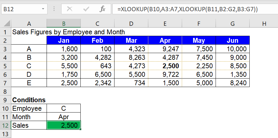
Case 2: Two-Way lookup usage
Suppose you want to search for the sales figure for a particular employee for a particular month then XLOOKUP function can be used as follows:


