How to Alternate Row Colors in Google Sheets
In this article, you will learn how to color rows with alternating patterns in Google Sheets. This Google Sheets function allows you to make your data table more visible and clear.
How to use the “Alternating color” function in Google Sheets
- Select an array you want to apply an alternating pattern.
- Go to the “Format” tab → “Alternating colors”.
- The pop-up menu shows up on the right side.
- Determine if you apply a pattern to “Header” and “Footer”.
- Choose a pattern you like out of default patterns, or customize your design.
- Click the “Done” button at the bottom right.
Steps 1 and 2

Steps 3 to 5

What is the alternative way of “Alternating colors”
You can use Conditional Formatting instead of Alternating colors to alternate row colors.
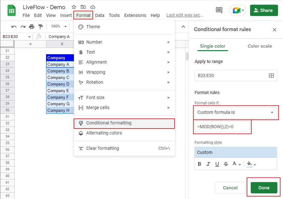
- Select the range you want to apply a pattern.
- Navigate to the “Format” tab → “Conditional formatting”.
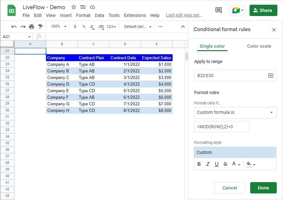
- Choose “Custom formula is” → Enter “=MOD(ROW(),2)=0”.
- Click the “Done” button at the bottom right.


You need to understand that you make the MOD function return 0 (where a row number is even) or 1 (when a row number is odd) by entering 2 as its divider and that the Conditional Formatting you define is applied where the MOD function returns 0. In the example, Conditional Formatting is effective for rows with even numbers.
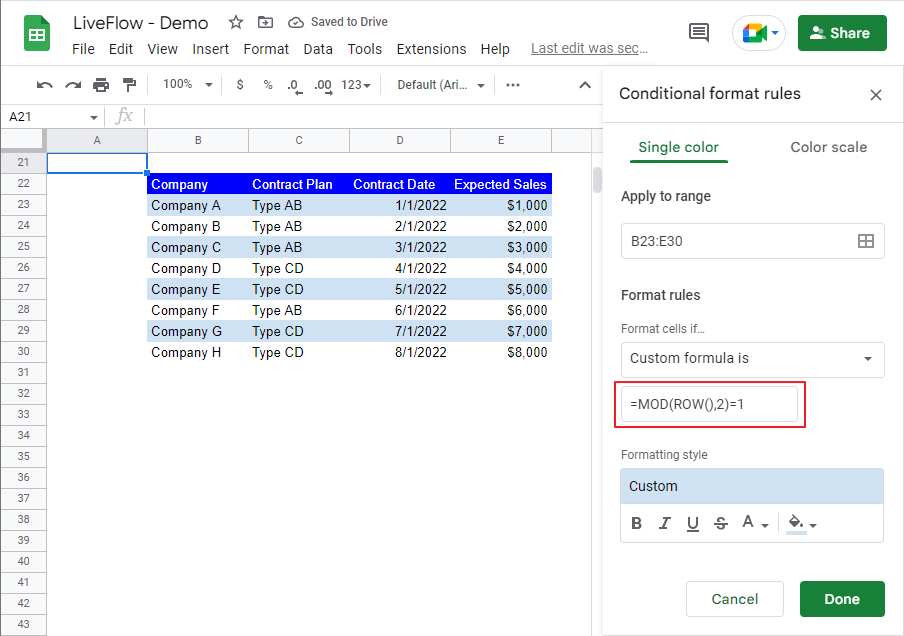
If you want to apply Conditional Formatting to rows with odd numbers, you can change the custom formula to “=MOD(ROW(), 2)=1”. You can see the outcome in the picture below.

How to alternate column colors in Google Sheets
Check this article: Alternate Column Colors in Google Sheets: Explained to learn how to add alternating colors to columns.

